SlicerDSpace

Diffusion MRI workflows in 3D Slicer. Source code Download video

Native diffusion space

Outputs from SlicerDSpace.

Representative maps, surfaces, pathways and networks from the available analysis routes. Each view highlights a different product in native diffusion space.

Complete result overview: anatomical priors, microstructure maps, four tractography methods, WMQL, TractCloud and WMA fiber bundles, and structural connectomes — Maps, cortical surfaces, fiber bundles and connectomes from the available analysis routes. Open full-size SVG

Choosing routes

Workflow overview.

Get started

From installation to your first result.

Install, run and review with your Agent. (Recommended)

Read the Skill

We provide an install-and-use Skill for SlicerDSpace. Give its SKILL.md to your local Agent to follow the project's setup, analysis and result-review workflow.

The prompts link to SKILL.md as the entry point. To install the Skill in your Agent, copy the complete slicerdspace folder with its references, scripts and templates.
Install and enable
Agent prompt
```
Read https://github.com/NeuroDMRI/SlicerDSpace/blob/main/.agents/skills/slicerdspace/SKILL.md.
Install and enable SlicerDSpace in my local 3D Slicer.
Set up the required dependencies and download the corresponding model weights.
```
Your Agent checks storage space and existing resources, waits for your choice and saves the path for later use. It prepares only the selected analyses. Confirm licenses and restarts when requested.

Use an existing installation

Replace the input and output paths, and choose the methods your study needs. This example requests DDParcel, CSD/ACT tractography and a structural connectome.

Analysis prompt

Read https://github.com/NeuroDMRI/SlicerDSpace/blob/main/.agents/skills/slicerdspace/SKILL.md.
Use SlicerDSpace to run DDParcel brain parcellation, CSD/ACT tractography and structural connectome construction for /path/to/subject; save results to /path/to/results.
Show me the plan and wait for confirmation before running. Afterwards, summarize the outputs and QC findings.

Or set up manually

Install the module

Start with 3D Slicer; the protocol reference is version 5.10. Clone the source and create a separate extension installation:
bash
```
git clone https://github.com/NeuroDMRI/SlicerDSpace.git
cd SlicerDSpace
python3 scripts/stage_slicer_extension.py \
  --install-root ~/SlicerDSpace-extension --slicer-version 5.10 \
  --link-mode copy
```
Replace 5.10 with the major/minor version shown in Slicer’s About dialog. The script stages the module and reports its installation directory.
Add the module path

Open Edit › Application Settings › Modules › Additional module paths. Add the expanded absolute path of ~/SlicerDSpace-extension/SlicerDSpace/lib/Slicer-5.10/qt-scripted-modules, matching the version you staged.

Install SlicerDMRI and PyTorch from Slicer’s Extension Manager. Add the separate UKFTractography extension if you plan to use UKF. Restart Slicer, then open Modules › Diffusion › SlicerDSpace.
Prepare the subject inputs

Enter a Subject ID and Subject root. For prepared inputs, use this layout; the output directory can remain empty to use the subject’s outputs/ folder.
```
sub-01/
  input/
    data.nii.gz
    bvals
    bvecs
    nodif_brain_mask.nii.gz   # optional; supply or generate
```
DWI and mask must share one voxel grid. The gradient count must match the DWI volume count, and motion-corrected images need the corresponding rotated gradients.

For DICOM or NRRD/NHDR, use Advanced settings › Regions & input import › Input import / conversion. Preview the import, then prepare the inputs before analysis.
Select methods and prepare their environment

For a small first run, select only Microstructure, clear the other products and keep DTI in its ... selector. For a fuller route, choose one or several algorithms beside each product. Advanced settings contains the model and tracking parameters.

Open Environment and installation › Prepare selected analysis environment. Confirm the required tools, models and resource terms. Downloads are checked and cached for reuse. If a restart is requested, restart and select Prepare again to continue.

Offline model resources, repair and manual path overrides are under More options. An existing reviewed mask avoids installing a mask-generation backend for the DTI-only route.
Run and inspect

Click Run SlicerDSpace. Missing fields are highlighted, and the log reports progress or a specific correction. Successful key products load automatically; DTI supplies FA and MD for inspection.

In Results and QC, select the run to inspect its checks and reload or replace products without duplicating scene nodes. Review mask coverage, alignment and method-specific QC before accepting results.

Command-line execution and cohort processing

From the checkout, use Slicer’s Python to check a DTI-only route. Replace the two absolute paths below:

bash

export SLICER_LAUNCHER="/path/to/Slicer"
export SUBJECT_ROOT="/path/to/sub-01"
"$SLICER_LAUNCHER" --launch PythonSlicer run_subject_pipeline.py \
  --subject-root "$SUBJECT_ROOT" --subject-id sub-01 --no-user-config \
  --targets microstructure --microstructure-stages dti --doctor

Repeat with --plan to inspect the processing plan, then --execute to run it. Keep the same method options for all three commands.

For example, --microstructure-stages dti,noddi selects two models; --tractography-backend csd_act,ukf selects two tracking variants; and --bundle-backend wmql,wma selects two bundle methods. Their input and dependency checks still apply.

For independent subjects, use scripts/run_batch_pipeline.py --batch-root /path/to/study --jobs 2 with your chosen analysis options. The GUI processes the current subject; the batch CLI manages separate outputs and logs.

Run times

Recorded run times, per module.

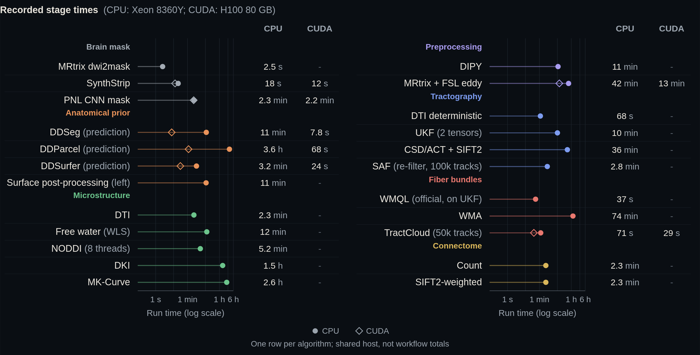
One row per algorithm, with CPU circles and open CUDA diamonds on a shared log-time axis. Aligned CPU and CUDA columns give both recorded times; the title names the repeat hardware. — Scoped stage times on a shared Linux host. Each algorithm occupies one row, with aligned CPU/CUDA time columns; seven routes have both device observations. A dash means no measurement for that device. Thread budgets differ by method and the devices are shared, so these are not controlled device speed ratios. Rows are not summed. SAF re-filters 100,000 existing tracks; TractCloud uses 50,000 tracks.

Performance

Runtime optimizations.

Measured comparisons for each operation, with its scope and implementation details.

Catalogue updated 30 October 2026

Download measurement data (JSON)

Different models and scopes are not ranked against each other. Ratios are reference time divided by optimized time.
Computation / scope	Type of change	Reference	Optimized	Measured ratio
Full brain / record 2026-10-29	Same-method implementation	15.64 min	11.89 min	1.32x23.99% less time
Upstream check Measured DIPY 1.12.1; latest stable on 29 October. The stable/head fitting definitions match qualified hashes; bounded protocol reuse is included in this full-brain pair. What changed Reuse protocol-only attenuation/spectrum/grid arrays in a bounded private cache, alongside diagonal-free weights and source-qualified tensor helpers. Reference Original installed DIPY WLS, not an earlier plugin. One numerical thread in both paths. Equivalence All 13 raw fit parameters, four maps/masks, affines, dtypes and automatic QC match. The same 116935 voxels remain excluded. Measured scope 740916 mask voxels; 288 measurements; automatic QC passes, anatomical review pending. Limits One subject, one pair on a shared Linux host; optimized first. OS caches were not flushed. Both calls include raw-parameter evidence export.
Complete module / record 2026-10-20	Same-method implementation	102.10 min	74.22 min	1.38x27.31% less time
Upstream check Author commit 4532b911386d: matches current HEAD and measured source bytes. What changed Bulk geometry copying and verified registration-input reuse reduce repeated Python/VTK traversal and preparation. Reference Original-author processing versus equivalent bulk/cache implementation, with identical UKF input and atlas. Equivalence All 74 anatomical-tract output files are byte-identical; source inputs and author code are unchanged. Measured scope Full registration and 74-tract output; no streamline downsampling introduced for timing. Limits One full-module pair on a shared Linux host. Matching files do not certify small-bundle sampling or anatomical validity. Later transform optimizations are not measured by this pair.
Full brain / record 2026-10-20	Native threads	29.15 min	5.19 min	5.61x82.19% less time
Upstream check AMICO 2.1.1 verified in both timed configurations; latest stable at review. Threads are already upstream functionality. What changed Use AMICO's existing native multithreading: one thread versus eight. Reference The same author implementation and model settings. This is a thread-configuration comparison, not a new algorithm. Equivalence NDI, ODI, IsoVF, RMSE, NRMSE and the tissue-validity mask match voxelwise, including affines. Measured scope Original 740916-voxel brain mask; fresh output directories. Limits One shared-host pair. Hardware-specific multithreading benefit; not a universal speed or whole-workflow guarantee.
64-voxel numeric chunk / record 2026-10-22	Python-port computation	1.73 s	1.09 s	1.58x36.70% less time
Upstream check Current MATLAB reference 9a213e1a5850; measured on current stable SciPy 1.18.1. This port-only comparison does not claim to outperform MATLAB or invent upstream native batching. What changed Reuse protocol/design checks and LAPACK workspace sizes while keeping the same pivoted QR and full b0 grid. Reference Current SciPy 1.18.1 public gelsy solver versus qualified direct-driver/cache use in the same Python port. NOT original MATLAB versus Python. Equivalence Raw coefficients, full curves, every map and validity decision match in all three subjects; both reference and batched solvers checked. Measured scope Three real 64-voxel chunks; 181 measurements; complete 200-201 point b0 grids; one numerical thread. Limits Table shows subject 100206 default-QR medians, three alternating repeats after warmup. Numeric chunks exclude input preparation and file export; not whole ROI or full brain. SciPy already supplies native batching.
64-voxel numeric chunk / incremental QR change / record 2026-10-29	Python-port computation	1.19 s	1.06 s	1.13x11.26% less time
Upstream check Recorded 29 October with SciPy 1.18.1; source/input checksums and one-thread settings are preserved. This is an incremental comparison within the Python port, following the qualified QR change. What changed Within each chunk, reuse non-b0 signals and their logarithms across the full synthetic-b0 scan; update only the candidate b0 column. Reference The preceding qualified-QR Python implementation versus added signal reuse; solver, grid, correction rules and one numerical thread stay fixed. Equivalence Original/corrected coefficients, complete curves, parameter maps, residuals and validity masks match exactly in all three acquisitions and both solvers. Measured scope Three acquisitions, 64 voxels each, 181 measurements and 200-201 synthetic-b0 samples. Reference-QR time falls 10.24-11.26%. Numeric computation only; input preparation and file export excluded. Limits Displayed medians use acquisition 1, selected consistently with the earlier QR record. Three alternating repeats after one warmup. Batched-path changes range from -1.50% to +3.07%, so signal reuse remains enabled only for the reference solver. These incremental timings overlap the earlier QR implementation and are not additive.
Native 24-cubed ROI / record 2026-10-22	Existing upstream capability	37.11 s	11.47 s	3.24x69.09% less time
Upstream check DIPY 1.12.1 is current stable at review. Array metrics already exist upstream; this is plugin integration, not an author-algorithm speedup. What changed Evaluate the author's existing array-capable kurtosis metrics once per block, avoiding repeated per-voxel result wrappers. Reference Previous plugin per-voxel integration versus existing DIPY array usage. No improvement over the author's native vectorized API is claimed. Equivalence All exported voxel arrays and affines match in three subjects, with three alternating repeats each. Measured scope Three subjects; three repeats per path; native-grid ROI, no resampling; DIPY 1.12.1 with SciPy 1.18.1. Limits Table shows subject 100307 medians. This adopts existing native DIPY functionality, not a new upstream algorithm improvement. No completed full-brain DKI pair; do not scale ROI times to whole brain.
Native 24-cubed ROI / record 2026-10-20	Workflow scheduling	43.95 s	24.63 s	1.78x43.96% less time
Upstream check Historical plugin scheduler comparison, not a latest-upstream algorithm performance claim. What changed Overlap independent model subprocesses after their shared inputs are ready; preserve downstream dependencies. Reference The same model computations, serial scheduling versus two concurrent workers. Equivalence All exported scalar and mask arrays match. Process startup is included. Measured scope Two independent models; CPU/memory-constrained scheduling; not full-brain timing. Limits One ROI pair. This reduces schedule wall time, not the cost of an individual scientific model. Default model concurrency remains one; memory/CPU budgets may prevent overlap.
Single substage / record 2026-10-20	Same-method implementation	134.29 s	2.48 s	54.06x98.15% less time
Upstream check Same immutable current WMA source audit as the full-module record. What changed Replace per-point Python geometry copying with equivalent bulk coordinate/topology operations. Reference Unmodified author filter on the full 1989106-streamline registration atlas. Equivalence Output coordinates/topology and fixed-seed samples match exactly. Measured scope Full registration-atlas length-filter substage only. Limits One full-atlas substage pair, not complete WMA. The large local ratio must not be multiplied by or added to the full WMA result.
1728-voxel ROI / record 2026-10-21	Same-method implementation	12.47 s	5.17 s	2.41x58.50% less time
Upstream check Measured DIPY 1.12.1 in Slicer; author NLS/residual/Jacobian source hashes match the dated stable-source audit. What changed Call source-qualified author NLS, residual and Jacobian bodies directly, removing repeated keyword-compatibility dispatch. Reference Installed original DIPY 1.12.1 serial NLS versus the same function bodies; one numerical thread in both paths. Equivalence All 13 raw parameters, exported maps, affine and QC decisions match in all three subjects. Measured scope Three native 12-cubed ROIs; 288 measurements; complete ROI stage including fresh export. Limits Subject 100307 medians, three alternating repeats after warmup. ROI, not full brain. These timings precede later WLS-initialization/helper changes and cannot be added to them.
1000 fibers x 15 points / record 2026-10-21	Same-method implementation	24.6 ms	0.322 ms	76.31x98.69% less time
Upstream check Author register_two_subjects.py SHA256 matches the 22 October WMA source audit; measured bulk vtkTransform path. What changed Use the same author vtkTransform with a bounded bulk point call, instead of one Python/VTK call per point. Reference Unmodified author point-transform loop versus bulk calls with the same float64 point order and transform. Equivalence All transformed points, complete small-optimizer trajectories and final transforms match in three subjects. Measured scope Three real-subject fixtures; explicit synthetic offset for the separate optimizer check. Limits Subject 100206 median of five point-transform repeats, not full registration. Small-optimizer gains were only about 1.27-1.28x; the point-kernel ratio cannot be applied to whole WMA.
20000 fibers x 15 points / record 2026-10-21	Same-method implementation	0.59 s	12.8 ms	45.84x97.82% less time
Upstream check Author fibers.py at 4532b911386d independently verified; native VTK array sampling, not a new registration algorithm. What changed Gather the same author nearest-neighbor fiber samples from VTK connectivity in bounded NumPy blocks. Reference Unmodified author FiberArray conversion versus equivalent bulk conversion; no interpolation or streamline reduction added. Equivalence All arrays, hemisphere flags and separate small-optimizer trajectories/transforms match in three subjects. Measured scope 20000 identical sampled fibers per subject; original nearest-neighbor rule and ordering. Limits Subject 100206 median of five conversion repeats. Not whole WMA; small-optimizer gains were only about 1.02-1.05x. Historical source sampling failures remain failed.
Three preparation calls / record 2026-10-20	Same-method implementation	8.90 min	3.01 min	2.96x66.17% less time
Upstream check Preserved same-author preparation pair. Source-qualified reuse, not a fresh latest-version benchmark. What changed Reuse verified deterministic atlas/subject length-filter results across seeds; keep fresh author random sampling. Reference Three original author preparation calls versus first cache fill plus reuse, with the same input and fixed seeds. Equivalence Bitwise-equal registration input signatures; source hashes unchanged Measured scope Three fixed-seed preparation calls, including first cache fill; not full WMA Limits One subject, one pair; includes initial cache construction. This overlaps WMA filtering and the full-module pair; savings cannot be added.
Four left-hemisphere overlays / record 2026-10-20	Inherited upstream optimization	13.38 s	3.52 s	3.80x73.70% less time
Upstream check Optimization inherited from DDSurfer c3b2d40; no plugin-original credit or latest-FreeSurfer speed claim. What changed Pack four overlays into one multi-frame mri_surf2surf call, sharing the same surface registration. Reference Four separate FreeSurfer commands versus one multi-frame command. Inherited from DDSurfer upstream c3b2d40, not plugin-original work. Equivalence Four byte-identical MGH outputs; 163842 vertices per overlay; source hashes unchanged Measured scope 100307 left hemisphere; four separate FreeSurfer commands versus one multi-frame command Limits One subject, command timing only; extra packing/validation excluded. Not surface reconstruction or a new FreeSurfer algorithm.
Three slabs / record 2026-10-20	Compressed data I/O	37.25 s	17.08 s	2.18x54.15% less time
Upstream check Generic compression/I/O control, not an improvement to a scientific estimator or an upstream-freshness claim. What changed Decode gzip once to temporary disk, then memory-map the same requested blocks; leave the source file unchanged. Reference Repeated compressed-array reads versus one sequential decode and disk-backed block reads; no indexed_gzip in this measurement. Equivalence Exact arrays and affine for all three slabs; unchanged input hash Measured scope Three real slabs including sequential decode. NOT a model-fit or full pipeline speedup. Limits One subject, one pair, uncontrolled OS page cache; needs temporary disk. I/O only, not model fitting; no universal storage-performance guarantee.

Read the complete optimization report

Methods & resources

What is integrated

Choose one or several methods beside each product. The workflow checks acquisition suitability, resolves dependencies and reuses shared preparation.

Methods, implementation and resources for the selected analysis routes.
Stage	Method	How it is integrated	Runtime / access	Papers
Input	DICOM / NIfTI / NRRD	Conversion, gradient validation and spatial checks.	dcm2niix or Slicer DWIConvert; supplied masks accepted	[36] [27] [28]
Brain mask	PNL CNN (default)	Author diffusion-CNN brain masking and registration.	Managed PNL runtime, weights and ANTs	[37] [38]
Brain mask	SynthStrip	Brain extraction with the author model.	Isolated runtime and weights	[32]
Brain mask	MRtrix3 dwi2mask	Native diffusion-volume masking.	MRtrix3	[29]
Preprocessing	MP-PCA	Random-matrix denoising and noise estimation.	DIPY or MRtrix3 dwidenoise	[39] [52] [53] [29] [30]
Preprocessing	Local PCA	Overcomplete local-PCA denoising.	DIPY; optional denoising choice	[40] [30]
Preprocessing	Patch2Self	Self-supervised diffusion-volume denoising.	DIPY; optional denoising choice	[41] [30]
Preprocessing	Gibbs removal	Local subvoxel-shift ringing correction.	DIPY or MRtrix3 mrdegibbs	[42] [29] [30]
Preprocessing	Volume registration	Between-volume motion correction and gradient rotation.	DIPY; does not perform FSL eddy correction	[30]
Preprocessing	FSL eddy	Eddy-current and motion correction.	MRtrix3 dwifslpreproc; FSL	[43] [29]
Preprocessing	FSL topup	Susceptibility-distortion estimation and correction.	FSL; reverse-phase data and acquisition metadata	[44] [29]
Microstructure	DTI (default)	LS/WLS tensor fitting; FA, MD, AD, RD, eigenvalues and trace.	SlicerDMRI	[45] [27] [28]
Microstructure	Free water	Free-water fraction and tissue-corrected FA/MD; WLS or NLS fitting.	DIPY; suitable multi-shell sampling	[4] [5] [6] [30]
Microstructure	NODDI / AMICO	NDI, ODI, IsoVF and fit residuals.	AMICO; suitable multi-shell sampling	[7] [31]
Microstructure	DKI	WLS/OLS fitting; MK, AK, RK, KFA, MKT, RTK and validity masks.	DIPY; shell, direction and design-rank checks	[8] [30]
Microstructure	MK-Curve	Correction curves, corrected kurtosis maps and metric-specific validity.	Bundled Python backend; DKI eligibility checks	[9]
Anatomical prior	DDSeg	Tissue labels and probabilities from converted PyTorch models.	PyTorch; DDSeg weights	[2]
Anatomical prior	DDParcel	Anatomical region inference with author-derived models.	PyTorch; weights and registration template	[3]
Anatomical prior	DDSurfer	Native white and pial mesh reconstruction.	PyTorch; DDSurfer weights	[1]
Anatomical prior	BRAINSFit registration	Template registration for eligible anatomical routes.	Slicer BRAINSFit / BRAINSResample	[51] [27]
Anatomical prior	Surface post-processing	Thickness, curvature, spherical registration and DK/Destrieux atlas mapping.	Licensed native component runtime; full suite optional	[33] [47] [48] [49]
Tractography	Response estimation	Dhollander three-tissue response estimation.	MRtrix3	[12] [13] [29]
Tractography	CSD / MSMT-CSD	Single- or multi-tissue fibre-orientation distributions.	MRtrix3; selected acquisition route	[11] [46] [10] [29]
Tractography	Multi-tissue normalization	Log-domain intensity and inhomogeneity normalization.	MRtrix3 mtnormalise	[17] [18] [29]
Tractography	iFOD2 / ACT (default)	Probabilistic tracking with DDSeg-derived tissue constraints.	MRtrix3; reviewed anatomical priors	[14] [15] [29]
Tractography	DTI deterministic	Tensor-based direction tracking with stopping criteria.	SlicerDMRI; DIPY	[45] [28] [30]
Tractography	UKF two-tensor	Automatic invocation of the official tracking CLI.	UKFTractography extension; SlicerDMRI	[19] [28]
Tractography	SAF	Surface-constrained short-association tracking and geometric filtering.	MRtrix3; post-processed native surfaces	[20]
Fiber bundles	WMQL (default)	Official bundle queries; optional subsets and regional cerebellar selections.	Author tract_querier; DDParcel labels	[21]
Fiber bundles	WMA	ORG, East-West or NABA atlas registration and clustering; automatic UKF handoff.	WMA; selected atlas; UKF reference route	[22] [23] [24] [26] [54] [55]
Fiber bundles	TractCloud	Author learned tract parcellation and bundle export.	PyTorch backend; model and centroids	[25] [22]
Connectome	Streamline count	Endpoint assignment to DDParcel nodes.	Python or eligible MRtrix3 backend	[50] [29]
Connectome	SIFT2-weighted count	FOD-informed weighting and matrix construction with matched tracks.	MRtrix3; corresponding tractogram and weights	[16] [29] [50]
Connectome	Scalar / length summaries	Mean FA, MD, ODI or another scalar; mean and total streamline length.	Python API; matched maps, nodes and tracks	[50] [29] [30]
Regional analysis	Selected-region analysis	Reuse maps for ROI statistics, filter tracks and extract node submatrices.	Advanced settings; workflow utility using completed outputs	[3] [30] [50]

Defaults: DTI, CSD/ACT and WMQL. Detailed parameters are in Advanced settings; selected dependencies are prepared separately under Environment and installation. External tools and model assets are not installed silently.

Implementation provenance and validation records document the backend versions and individual test scopes.

SlicerDSpace

Film

Outputs from SlicerDSpace.

Workflow overview.

From installation to your first result.

AInstall, run and review with your Agent. (Recommended)

Read the Skill

Install and enable

Use an existing installation

BOr set up manually

Install the module

Add the module path

Prepare the subject inputs

Select methods and prepare their environment

Run and inspect

CCommand-line execution and cohort processing